Intraday Trend Following and Conditional Mean Reversion
Yanyi Huang
Abstract
This study examines whether transparent intraday trend-following and conditional mean-reversion rules can generate statistically robust net returns in the Invesco QQQ Trust (QQQ), and whether those rules can be translated into a resilient broker-facing trading process. Two trend strategies are considered. The first combines exponential moving-average direction, MACD confirmation, ADX trend strength, and a volatility-expansion filter. The second compares a short volume-weighted moving average with a longer price average. A third strategy enters Bollinger %B mean-reversion trades only when a rolling Hurst estimate or variance-ratio statistic indicates a reversion-compatible state.
Adjusted regular-session OHLCV data are aggregated to 15-minute, 30-minute, hourly, and daily bars. The primary 30-minute experiment uses a chronological training period (2015–2020), validation period (2021–2022), and untouched test period (2023–2025). Parameters are selected on training data only, signals are executed one bar later, and returns are reported after explicit commission, spread, and slippage assumptions. Information coefficients, mean-return t-tests, Deflated Sharpe Ratios, parameter sensitivity, filter ablations, and cost stress tests are used to distinguish statistical evidence from data-mined performance.
None of the three 30-minute strategies produces positive out-of-sample net performance. Test Sharpe ratios are −1.573 for the EMA–MACD–ADX strategy, −0.633 for the volume-weighted ratio strategy, and −0.911 for conditional Bollinger mean reversion. Deflated Sharpe probabilities are correspondingly close to zero. Costs are economically important, although weak or negative gross performance also contributes to failure. Hourly and daily ratio diagnostics are more favourable, but these full-sample comparisons are not treated as out-of-sample evidence.
The research system is extended to an Interactive Brokers paper-trading architecture with deterministic order identifiers, an explicit order state machine, ClickHouse event and fill storage, position reconciliation, risk limits, health checks, and fail-closed behaviour. A deterministic 20-trading-day replay completed 259 signal cycles and 10 simulated fills. The backtests reject all three primary profitability hypotheses. The execution work instead shows that the same signals can be routed through a broker-facing process that detects stale data, duplicate events, and position mismatches before adding risk.
Keywords: algorithmic trading; trend following; mean reversion; transaction costs; IBKR; execution risk; Deflated Sharpe Ratio
1. Introduction
This project tests whether three transparent intraday rules survive transaction costs and out-of-sample evaluation on QQQ. Short-horizon strategies are exposed to turnover, spreads, slippage, stale data, partial fills, duplicate orders, and differences between broker status messages and actual positions. The research therefore evaluates both the historical signal and the broker-facing controls needed to run it [1].
This paper addresses the following research question:
Can transparent intraday trend-following and conditional mean-reversion rules generate statistically robust net returns in QQQ, and can those rules be executed reliably under realistic broker and operational constraints?
QQQ is selected because it is a heavily traded, technology-weighted exchange-traded fund with a long trading history [2]. This study uses it as a test instrument for trend persistence and short-horizon reversion. SPY is used as the systematic benchmark. The primary bar interval is 30 minutes, while 15-minute, hourly, and daily data provide timeframe diagnostics.
Four hypotheses are specified before examining the untouched test period:
- H1: EMA and MACD directional agreement, conditioned on ADX strength and expanding Bollinger bandwidth, produces positive out-of-sample net returns.
- H2: a volume-weighted short/long price ratio has positive out-of-sample predictive and economic value.
- H3: Hurst and variance-ratio gating improves Bollinger %B mean reversion.
- H4: transaction costs materially reduce short-horizon strategy performance.
The implementation combines a custom next-bar backtester, explicit transaction-cost attribution, IC and Deflated Sharpe diagnostics, and train-only PCA. The same repository contains an IBKR Paper execution path that reconciles executions, orders, positions, and account data instead of relying on a single broker status callback.
2. Literature Review
Trend following assumes that price changes can persist over an economically useful horizon. Time-series momentum evidence has been documented across liquid futures and asset classes [3], while systematic implementations emphasise volatility scaling, forecast normalisation, diversification, and cost control [4]. EMA cross-overs and MACD are practical transformations of the same broad idea: recent information receives greater weight than older information. ADX adds a direction-neutral measure of trend strength, allowing the trading rule to distinguish directional movement from range-bound noise [5,6].
Mean reversion instead assumes that deviations from a local equilibrium are temporary. Bollinger Bands define a rolling volatility envelope around a central estimate [7]. The associated %B statistic standardises the location of price within the envelope. A mechanical %B rule remains vulnerable when a persistent trend drives price outside the band, so this paper conditions new entries on Hurst and variance-ratio diagnostics. The variance-ratio framework tests whether multi-period return variance is consistent with a random walk [8,9]. These diagnostics are inherently noisy and lagging; they are therefore treated as state filters rather than standalone forecasts.
Backtest selection introduces a separate problem. Trying many related rules increases the probability that the best in-sample Sharpe ratio is a sampling artefact. The Deflated Sharpe Ratio adjusts the observed Sharpe for non-normality and the number of trials [10], complementing chronological holdouts and embargoed training observations. Technical indicators are therefore not assumed to work merely because they have familiar names. Their direction, stability, turnover, and cost-adjusted out-of-sample behaviour must be demonstrated [11].
Execution literature also distinguishes a desired portfolio from a realised one. Order type, time-in-force, routing, queue position, spreads, latency, partial fills, and message sequencing all influence implementation shortfall [1]. The execution component of this project consequently uses broker-independent order models and a reconciliation layer around IBKR Paper rather than accepting a single status callback as truth.
3. Data and Exploratory Design
3.1 Instruments and sampling
The primary instrument is QQQ and the benchmark is SPY. The source files are a commercial
historical market-data set purchased from a third-party seller through the Taobao
marketplace. The files contain split- and dividend-adjusted minute-level OHLCV observations,
but the seller did not provide independently verifiable exchange-level data lineage; they
are therefore not represented as official exchange records. Seller identity, purchase
records, and transaction evidence are retained privately. For examiner reproducibility,
QQQ and SPY files under data/market/processed/ and data/market/raw/ are included in
the submission package; other symbols present in the local archive are omitted. The
observations are aggregated within the US regular trading session.
Bars are labelled by completion time. The principal sample contains 35,881 valid
30-minute QQQ observations from 2 January 2015 to 30 December 2025. The automated audit
found no duplicated timestamps, missing OHLCV values, or invalid OHLC relationships.
Six same-session gaps were identified and retained as explicit source-data limitations
rather than silently imputed.
The chronological split is:
- training: 2015–2020, with the last 13 overlapping observations embargoed;
- validation: 2021–2022;
- untouched test: 2023–2025.
The resulting counts are 19,583 training, 6,536 validation, and 9,749 test observations. The 13 embargoed observations remain in the full data set but are excluded from all three split-level metric masks, so the split counts sum to 35,868 rather than 35,881. The test period is not used to select indicators or parameters.
3.2 Point-in-time controls
All indicators use backward-looking rolling or exponentially weighted calculations. A signal formed at the close of bar $t$ becomes an executable target only on bar $t+1$. No contemporaneous close is used both to create and execute a signal. Data-loading routines validate ordering, duplicates, OHLC consistency, completeness, and bar count. Live-bar validation additionally rejects stale, future-dated, mismatched-symbol, or non-finite observations.
The available source is aggregated market data rather than a reconstructed order book.
Consequently, the study cannot estimate queue position or transient impact from true
exchange ticks. As a brief-aligned diagnostic, one-minute adjusted OHLCV rows are treated
as the finest sampling grid and aggregated into tick-proxy (fixed event count), volume, and
dollar bars for calendar year 2019; thresholds are matched to median 30-minute activity.
These event-based sampling constructions follow the project brief and standard financial
machine-learning terminology [12,13]. They are reported under outputs/part1/event_bars/
and do not replace
the primary 30-minute time-bar experiment or its parameter selection. Volume weighting in
Trend-B remains the practical non-price-only extension on the primary clock.
4. Methodology
4.1 Trend Strategy A: EMA–MACD–ADX
For closing price $P_t$, the exponentially weighted mean with span $n$ is denoted $\operatorname{EMA}_n(P_t)$. The directional component is
$$ D_t^{\mathrm{EMA}}=\operatorname{sign}\left( \operatorname{EMA}{n_f}(P_t)-\operatorname{EMA}{n_s}(P_t) \right). $$
MACD confirmation is fixed at the standard $(12,26,9)$ construction throughout [5]; it is not re-parameterised when the EMA direction pair changes. The implementation divides the line and signal by the current close for scale invariance; only the histogram sign is used for confirmation:
$$ D_t^{\mathrm{MACD}}=\operatorname{sign}(\mathrm{MACD}_t-\mathrm{Signal}_t). $$
A trade is permitted only when the two directions agree, ADX exceeds a threshold, and the 20-period Bollinger bandwidth exceeds its 130-bar rolling quantile. The training grid searches EMA direction pairs $(5,20)$, $(8,32)$, and $(12,26)$ against that fixed MACD confirming horizon, together with ADX thresholds 20 and 25 and bandwidth quantiles 0.5 and 0.6. The selected configuration is $(12,26)$, ADX 20, and bandwidth quantile 0.6, so the reported rule uses a shared EMA/MACD horizon. ADX follows Wilder’s direction-neutral trend-strength construction [6], while BandWidth follows Bollinger’s volatility-envelope framework [7].
4.2 Trend Strategy B: volume-weighted ratio
This short/long ratio design implements the corresponding project-brief requirement [12]. The short estimate is a volume-weighted moving average:
$$ \mathrm{VWMA}t(n_f)= \frac{\sum{i=0}^{n_f-1}P_{t-i}V_{t-i}} {\sum_{i=0}^{n_f-1}V_{t-i}}. $$
It is compared with a longer simple average:
$$ R_t=\frac{\mathrm{VWMA}_t(n_f)}{\mathrm{SMA}_t(n_s)}. $$
The strategy is long when $R_t>1+\varepsilon$, short when $R_t<1-\varepsilon$, and flat inside the neutral zone. The training grid uses long windows 20, 40, 65, and 130; $\varepsilon$ values 0.001, 0.002, and 0.005; and both volume-weighted and price-only short estimates. The selected 30-minute rule uses a five-period VWMA, 130-period long mean, and $\varepsilon=0.005$.
4.3 Conditional Bollinger mean reversion
For rolling centre $\mu_t$, standard deviation $\sigma_t$, and width $k$ [7],
$$ U_t=\mu_t+k\sigma_t,\qquad L_t=\mu_t-k\sigma_t, $$
$$ B_t=\frac{P_t-L_t}{U_t-L_t}. $$
A value below zero initiates a long position and a value above one initiates a short position. Positions are stateful: a long exits when price reaches or exceeds the centre, and a short exits when price reaches or falls below it. This is materially different from recalculating a signed Z-score position every bar.
New entries are allowed when either [8,9]
$$ H_t < 0.5-\delta $$
or
$$ \mathrm{VR}_t(q)<1-\varepsilon, \qquad \mathrm{VR}(q)=\frac{\operatorname{Var}(r_t^{(q)})} {q\operatorname{Var}(r_t^{(1)})}. $$
The gate is deliberately an inclusive OR rather than a joint AND: either diagnostic may authorise an entry when the other is inconclusive. On outside-band candidates under the selected primary rule, this still admits most observations (about 83% in training and 85% in the test period), so the filter is a soft regime screen rather than a tight selector. The primary train-only search evaluates $q\in2,5,10$ jointly with the Bollinger window, width, and centre estimator. The selected model uses a 20-period exponentially weighted centre, $k=2$, a 130-period Hurst window, $\delta=0.03$, $q=5$, and variance-ratio tolerance 0.05.
4.3.1 Post-hoc enhanced design
After completing the primary experiment, an enhanced Bollinger specification was constructed as a post-hoc extension of the project brief [12]. It retains an EWMA centre and volatility and explicitly computes the standardised deviation and relative bandwidth:
$$ Z_t=\frac{P_t-\mu_t}{\sigma_t}, \qquad W_t=\frac{U_t-L_t}{\mu_t}=\frac{2k\sigma_t}{\mu_t}. $$
The enhancement modifies entry permission only; direction and exit rules are unchanged. Price must first lie outside a band. If $|Z_t|>3.5$, the observation is treated as an extreme shock or strong trend and no contrarian tail entry is placed. The causal percentile of $W_t$ over the previous 130 bars must lie between 20% and 80%: below 20% is classified as a squeeze and above 80% as a high-volatility/trending state. A three-bar rise in bandwidth combined with three consecutive closes outside the same band is also classified as ride-the-band behaviour [7]. The final permission is
$$ \mathcal{G}_t= \mathcal{G}^{H/VR}_t \cap\mathcal{G}^{BW}_t \cap|Z_t|\leq3.5. $$
Here $\mathcal{G}^{H/VR}_t$ remains the Hurst/VR gate. All gates affect new entries only; an existing position retains the centre-line exit, avoiding forced execution at an exceptional price. The enhanced model compares only $(n,k)\in{20,40}\times{1.5,2.0}$ on training data and fixes the other thresholds in advance. Because this design followed observation of the primary test result, it is reported separately as a post-hoc robustness experiment and does not replace the pre-specified primary result.
4.4 Auxiliary features and PCA
A compact feature panel covers momentum, volatility-scaled momentum, EWMAC, MACD, ADX, ATR, realised and downside volatility, drawdown, Bollinger %B and bandwidth, VWMA distance, volume anomalies, RSI, Hurst, variance ratio, QQQ–SPY relative momentum, and rolling beta. The panel is intentionally limited rather than expanding to hundreds of highly correlated parameterisations.
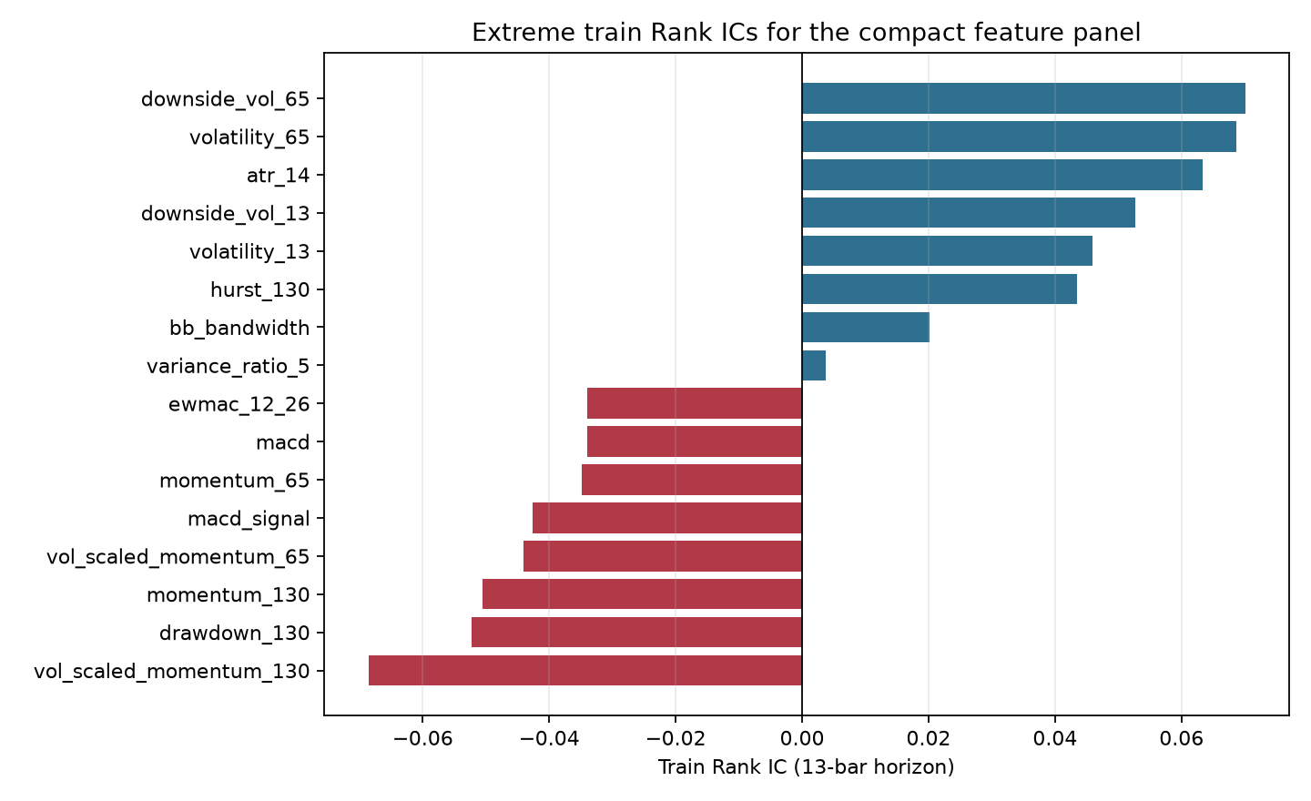
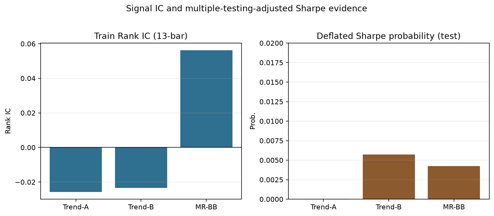
The largest absolute 13-bar rank ICs in training are modest: downside volatility over 65 bars (0.070), realised volatility over 65 bars (0.069), volatility-scaled 130-bar momentum (−0.069), and ATR (0.063). These magnitudes suggest weak but non-zero conditional relationships, not immediately tradable forecasts. Figure 1 summarises the extreme ends of the Rank-IC distribution: volatility and ATR dominate the positive side, while several momentum constructions sit on the negative side. The pattern warns against treating “momentum” as uniformly predictive at the 30-minute horizon.
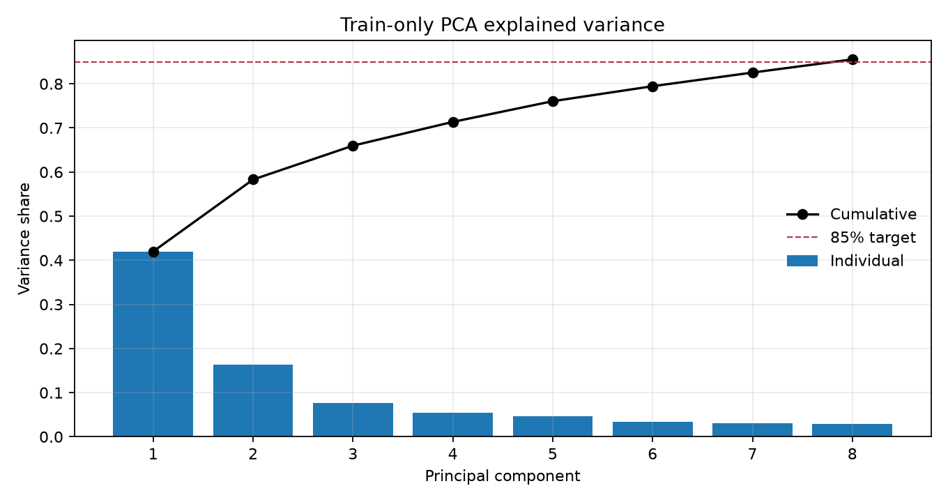
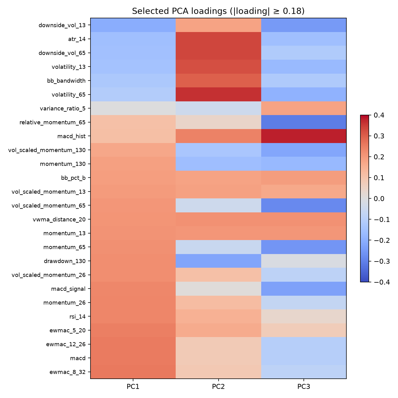
PCA is fitted after train-only median imputation and standardisation [14]. PC1 explains 42.0% of feature variance and loads positively on EWMAC, MACD, momentum, RSI, and drawdown while loading negatively on volatility measures. It can therefore be interpreted approximately as a trend/risk-on axis. PC2 explains 16.3% and places larger positive weights on realised volatility, ATR, and Bollinger bandwidth. Eight components are required to explain 85.5% of variance.
The selected loadings in Figure 3 make the redundancy explicit: many familiar trend indicators load on the same dominant axis. PCA scores are not used to trade or select strategy parameters.
Feature–forward-return information coefficients and train-only parameter selection measure whether each transparent signal predicts subsequent returns under a chronological split. Train-only PCA summarises collinearity among indicators; it is not a trading model. More flexible black-box models were not used because the available sample and the narrow single-instrument question do not justify their additional leakage and model-selection risk. Section 10 separately tests a QQQ–SPY linear combination.
4.5 Custom backtest and cost model
The custom engine maps each signal into a volatility-targeted position, following the standard systematic-trading rationale for volatility scaling [4]:
$$ w_t=\operatorname{clip}\left( s_t\frac{\sigma^\star}{\widehat{\sigma}t}, -w{\max},w_{\max} \right), $$
where $\sigma^\star=10$ annual volatility, $w_{\max}=1$, and $\widehat{\sigma}t$ is an exponentially weighted return volatility estimate with span 64. Desired position $w_t$ is shifted by one bar before return attribution: a signal formed at the close of bar $t$ applies to the close-to-close return from $t$ to $t+1$. Position-change events in the trade log are timestamped at Open$(t+1)$ for operational readability, but P&L attribution remains close-to-close rather than open-to-open. Turnover is $|w_t-w{t-1}|$. Baseline one-way cost is five basis points: one basis point commission, two spread, and two slippage. Cost stress multiplies all components by two and three.
The study reports gross and net return, CAGR, annualised volatility, Sharpe, Sortino, maximum drawdown, Calmar, turnover, and trade count; the Sharpe measure follows its standard formulation [15]. Pyfolio-reloaded independently generates a daily risk tear sheet from exported returns, positions, transactions, and SPY benchmark returns [16].
4.6 Statistical validation
Signal IC and rank IC are measured against one- and 13-bar forward returns separately on training, validation, and test observations, as required by the project brief [12]. Test-period mean net returns are evaluated with a two-sided t-test. The Deflated Sharpe Ratio accounts for all pre-specified train-only trials across the three primary strategies, not merely the winning strategy’s grid, and for return skewness/kurtosis. The enhanced Bollinger grid is listed separately as post-hoc [10,11]. Per-strategy gross return, commission, spread, slippage, and net-return drag are exported as a cost-attribution table. Filters are assessed by comparing the selected strategy with a matched version that removes the filter. Results are interpreted conservatively: validation improvement does not authorise subsequent test-period redesign.
4.7 Numerical techniques utilised
Table 1 summarises the numerical methods implemented in code. The list is intentional: each row maps to a module used in the primary experiments, diagnostics, or execution evidence, rather than to an exhaustive survey of possible estimators.
| Technique | Role in this study | Main accuracy / variance notes |
|---|---|---|
| SMA / EWMA rolling mean and volatility | Centres and widths for Bollinger rules; vol targeting input | Longer spans reduce variance but increase lag (bias toward old regimes) |
| MACD $(12,26,9)$ histogram sign | Fixed confirmation for Trend-A | Horizon not re-optimised with the EMA grid; reduces free parameters |
| Wilder ADX | Trend-strength filter | Direction-neutral; noisy on short bars |
| Bollinger %B / BandWidth | MR location; Trend-A expansion filter | %B outside $[0,1]$ triggers MR candidates; BandWidth quantile needs long warm-up |
| Rolling Hurst (log-variance vs lag) | Soft MR regime screen | Simplified estimator; high variance, slow to adapt |
| Rolling variance ratio $\mathrm{VR}(q)$ | Soft MR regime screen (OR with Hurst) | Inclusive OR admits most outside-band bars; diagnostic, not a formal test |
| Train-only OLS hedge $\hat\beta$ | QQQ–SPY log-spread construction | Frozen after train to avoid leakage; misspecification bias if co-movement changes |
| Rolling OU / Bollinger on spread | Relative-value entry thresholds | Same window-length trade-off as single-name bands |
| Next-bar backtest + turnover costs | Economic evaluation | Close-to-close PnL; Open$(t+1)$ only labels trades; fixed bps omit impact |
| Volatility targeting | Position scaling to 10% annual vol | Caps leverage; does not create alpha |
| Cost attribution + $1\times$–$3\times$ stress | H4 / cost channel | Proportional stress; not a microstructure calibration |
| Filter ablations | Causal contribution of gates | Matched test comparison; does not rescue negative Sharpe |
| Cross-timeframe replay | Sampling robustness | Full-sample under 30m params — hypothesis-generating only |
| IC / Rank IC, $t$-test, Deflated Sharpe | Statistical validation | DSR adjusts for trial count and non-normality; IC paths show temporal variance |
| Train-only PCA | Collinearity diagnostic | Not traded; eight components for 85% variance |
| Tick / volume / dollar bar proxies | Brief-aligned sampling diagnostic | Built from 1-minute OHLCV, not exchange ticks |
| Event sequencer (Rust / Python) | Broker-message order and dedupe | Fail-closed on conflicting IDs for live submit |
Table 1. Numerical techniques coded and used in the reported experiments.
5. Empirical Results
Section 5 compares the three primary rules out of sample, then stress-tests the economic and filter assumptions: proportional cost multipliers, matched filter ablations, cross-timeframe diagnostics, and the labelled post-hoc enhanced Bollinger exercise. Before the tables, Subsection 5.0 states how bias, variance, and accuracy of the estimators limit what the plots can claim.
5.0 Statistical and computational properties
The empirical plots should be read as statements about estimator noise and design bias, not only as performance charts.
Bias. Fixed five-basis-point one-way costs ignore time-varying spreads and impact, so gross-to-net gaps can be optimistic or pessimistic depending on the true liquidity regime. Close-to-close return attribution and the soft Hurst/VR OR gate both tilt the design: the former is an accounting convention rather than open-to-open mark-to-market, and the latter admits most outside-band candidates (Section 4.3), so “filtered” mean reversion is only weakly screened. Train-only parameter selection and the 13-bar embargo reduce look-ahead bias; they do not remove model misspecification.
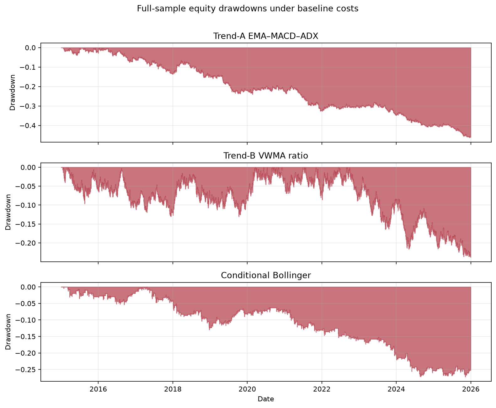
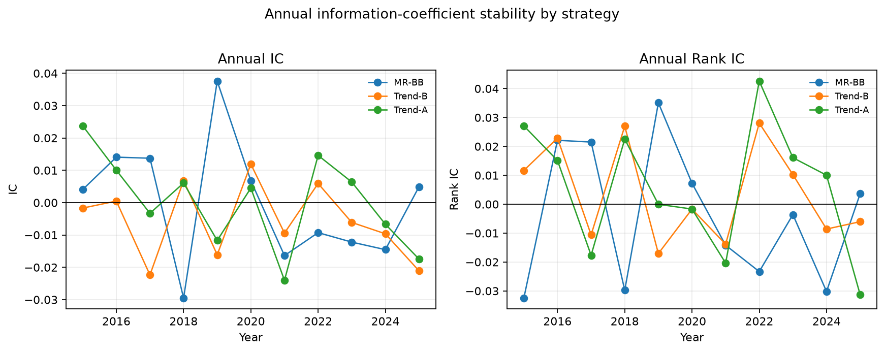
Variance. Short-horizon signals and rolling Hurst/VR estimates are high-variance objects. Figure 8 shows annual IC and Rank IC changing sign repeatedly, which is the statistical counterpart of unstable directional forecasts. High turnover in Trend-A and Trend-B amplifies path noise in equity and drawdown (Figures 4–5). Figure 1’s Rank-IC extremes are modest in absolute level, consistent with weak signal-to-noise rather than a sharp predictive edge.
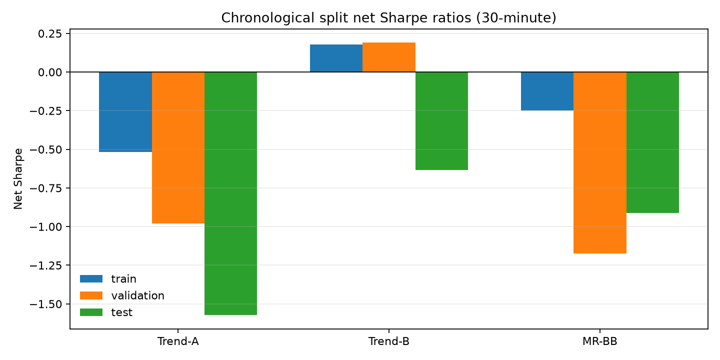
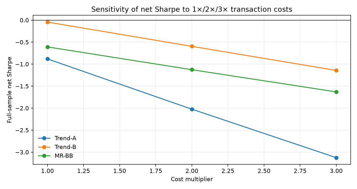
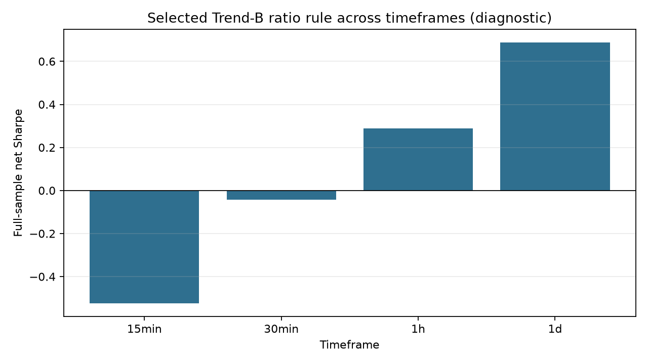
Accuracy and convergence. Lengthening estimation windows improves stability at the cost of lag: PCA needs eight components to reach 85% of feature variance (Figures 2–3), illustrating redundancy rather than a low-dimensional trading factor. Split Sharpes in Figure 6 show that even Trend-B—the only primary rule with positive train and validation Sharpes—fails to carry that success into a positive test Sharpe; Trend-A and MR-BB are already weak in training and worsen out of sample. Cost stress (Figure 9) shows that raising the one-way cost multiplier from $1\times$ to $3\times$ deepens net losses, while the $1\times$ baseline itself never yields a robustly positive net Sharpe for these rules—and MR-BB remains negative even gross. Cross-timeframe Sharpes (Figure 11) improve at hourly/daily horizons in a full-sample sense, but that pattern is not an independent OOS convergence result under re-selected parameters.
5.1 Out-of-sample performance
| Strategy | Test return | Test Sharpe | Test max drawdown | Test turnover |
|---|---|---|---|---|
| EMA–MACD–ADX | −21.92% | −1.573 | −25.23% | 382.28 |
| VWMA ratio | −17.43% | −0.633 | −21.85% | 328.09 |
| Conditional Bollinger | −11.20% | −0.911 | −14.23% | 126.04 |
None of the primary hypotheses concerning positive 30-minute OOS net returns is supported. The benchmark Buy and Hold strategy returned 545.7% over the full period with a Sharpe ratio of 0.925, although this is not a risk- or exposure-matched comparison.
Figure 4 places the three net equity paths against Buy and Hold. Buy and Hold grows by more than a factor of six, while all three strategies finish below unity after baseline costs. Trend-B is the least destructive of the three active rules, but it still decays after 2022. Trend-A and conditional Bollinger both grind lower across the sample.
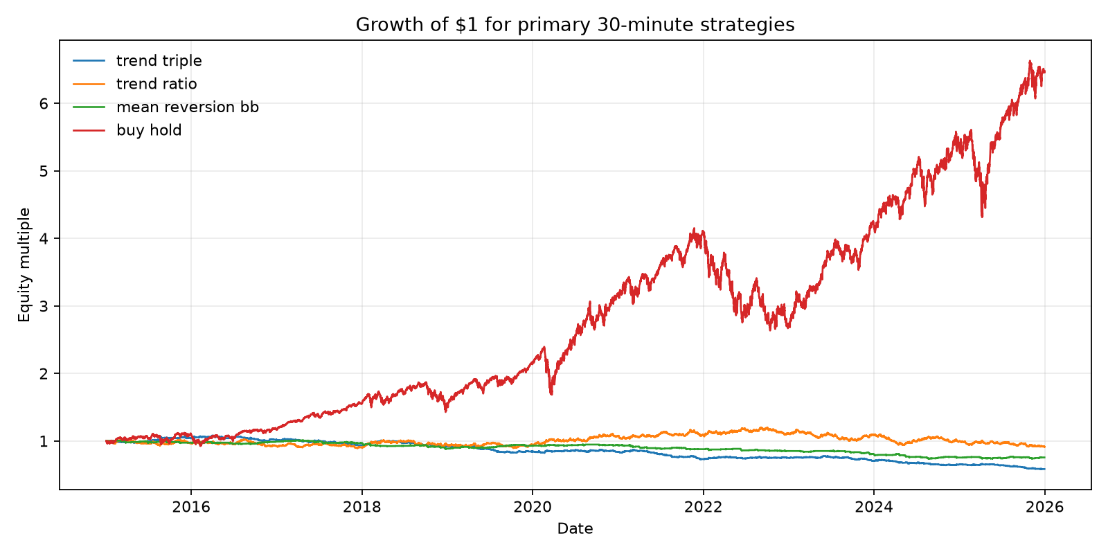
Figure 5 shows the corresponding drawdown paths. Trend-A and Trend-B experience deep and persistent drawdowns under high turnover, while Bollinger drawdowns are smaller in amplitude but still chronic. Figure 6 then decomposes net Sharpe by chronological split. Trend-B is the only rule with positive train and validation Sharpes, yet the untouched test Sharpe collapses to −0.633. Trend-A and MR-BB are already weak in training and worsen out of sample.
The EMA–MACD–ADX test mean is significantly negative under an unadjusted t-test ($t=-2.71$, $p=0.0067$), indicating a persistent loss under the zero-mean IID approximation. The ratio and Bollinger test means are not significantly different from zero at 5% ($p=0.275$ and $p=0.116$, respectively).
Deflated Sharpe probabilities are 0.0000015, 0.00113, and 0.000204 for the three strategies (Figure 7). These values provide no evidence that the observed test Sharpe ratios exceed a multiple-testing-adjusted benchmark. Annual IC paths in Figure 8 are likewise unstable and frequently change sign, reinforcing the conclusion that the directional signals are not robust through time.
5.2 Costs and gross performance
Transaction costs are material, but they are not the sole cause of failure. Across the full sample, the EMA–MACD–ADX strategy has a positive gross return of 16.2% but a net return of −41.7%; doubling costs lowers net return to −70.7%. The ratio strategy has a gross return of 59.6% but a baseline net return of −8.7%; doubling costs produces −47.8%. The mean-reversion strategy is already negative before costs (gross −4.5%) and falls to −24.4% net at baseline costs. H4 is therefore supported: costs materially damage all short-horizon strategies, while the mean-reversion rule also suffers from weak gross alpha.
Figure 9 makes the cost channel explicit. Raising the one-way cost from 1× to 3× pushes all three full-sample net Sharpes deeper into negative territory. Trend-B starts closest to zero under baseline costs and is therefore the most sensitive to the cost multiplier; MR-BB remains negative even before costs, so the stress test mainly amplifies an already weak signal.
5.3 Filter ablations
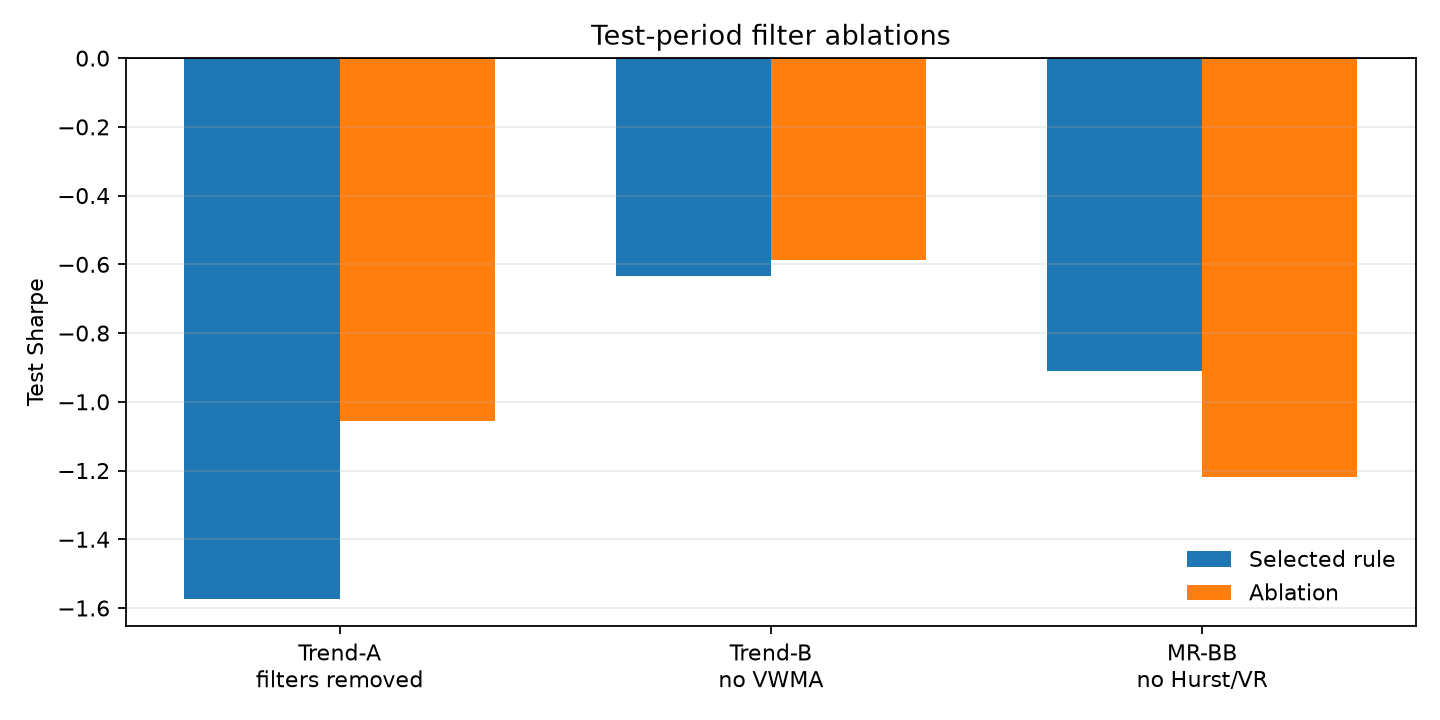
Removing ADX and bandwidth filters improves the Trend-A test Sharpe from −1.573 to −1.055, although performance remains unacceptable. Replacing the VWMA short estimate with a price-only estimate changes the ratio Sharpe from −0.633 to −0.587; volume weighting does not improve OOS performance. Removing Hurst/VR gating worsens Bollinger Sharpe from −0.911 to −1.218. The state filter therefore improves relative mean-reversion performance, but it does not create a profitable strategy. H3 receives limited relative support, whereas H1 and H2 are rejected in their current forms. Figure 10 compares each selected rule with its matched ablation on the untouched test period.
5.4 Timeframe diagnostics
Applying the selected ratio specification across full samples produces Sharpe ratios of −0.524 on 15-minute bars, −0.044 on the primary 30-minute full sample, 0.289 on hourly bars, and 0.688 on daily bars (Figure 11). This pattern is consistent with lower-frequency signals experiencing less microstructure noise and turnover [1]. It is not, however, valid OOS proof because these figures are full-sample diagnostics and the parameters originated from the 30-minute experiment. A future study must repeat train/validation/test selection independently for each timeframe.
5.5 Post-hoc enhanced Bollinger robustness test
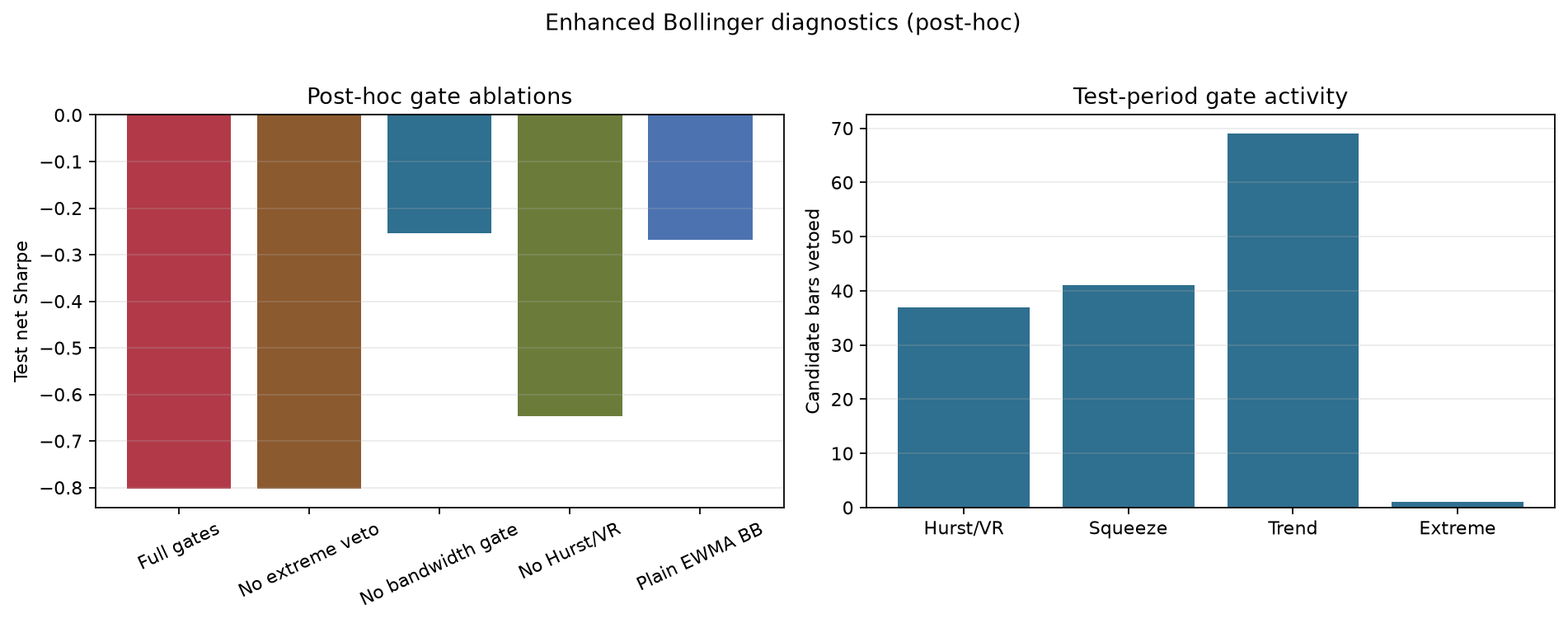
After observing the primary test result, an enhanced specification was implemented as an extension of the project brief [12]. It retains EWMA Bollinger %B entries and center-line exits, but adds three entry-only controls: a trailing BandWidth percentile gate, a rising-bandwidth ride-the-band veto, and an extreme-tail veto above 3.5 standard deviations. Hurst/VR remains a regime filter rather than a directional signal. Because the 2023–2025 outcome was already known, this is explicitly a post-hoc robustness exercise and not a new untouched OOS test [10,11].
Train-only selection chose a 40-bar EWMA center and width 2.0. Relative to the original MR-BB, test Sharpe improved from −0.911 to −0.803, test return from −11.2% to −9.8%, and maximum drawdown from −14.2% to −11.7%. Turnover fell from 126.0 to 68.3. Notably, gross return deteriorated from −5.42% to −6.70%; the net improvement comes from lower trading costs rather than stronger predictive alpha. The improvement is therefore real in a relative descriptive sense, but the strategy remains unprofitable.
| Test-period version | Net return | Gross return | Net Sharpe | Max drawdown | Turnover |
|---|---|---|---|---|---|
| Original MR-BB (20-bar EWMA) | −11.20% | −5.42% | −0.911 | −14.23% | 126.04 |
| Full enhanced rule (40-bar EWMA) | −9.84% | −6.70% | −0.803 | −11.69% | 68.27 |
Table 2. Descriptive comparison of original and enhanced Bollinger rules over the 2023–2025 test period. The enhanced rule is a post-hoc analysis.
The gate ablations in Figure 12 are more important than the headline comparison. Removing the BandWidth gate improves test Sharpe to −0.253, removing Hurst/VR improves it to −0.646, and the plain 40-bar EWMA Bollinger version records −0.268. The 3.5-sigma veto changes no test-period performance because it blocks only one candidate bar and that bar does not alter the realised position path. Thus the slower 40-bar estimator and lower turnover explain most of the improvement over the original 20-bar rule; the additional gates do not earn their keep in this sample. This does not overturn H3 on the primary MR-BB rule (Section 5.3), where removing the pre-specified Hurst/VR OR gate worsens the test Sharpe; the enhanced ablations are a different, already multi-gated 40-bar object and remain explicitly post-hoc.
| 40-bar EWMA ablation | Test net return | Test gross return | Test Sharpe | Test max drawdown |
|---|---|---|---|---|
| All gates | −9.84% | −6.70% | −0.803 | −11.69% |
| No extreme veto | −9.84% | −6.70% | −0.803 | −11.69% |
| No BandWidth gate | −4.26% | +1.42% | −0.253 | −8.79% |
| No Hurst/VR | −8.97% | −5.00% | −0.646 | −11.41% |
| Plain EWMA Bollinger | −4.80% | +1.64% | −0.268 | −10.05% |
Table 3. Matched gate ablations for enhanced Bollinger. All figures are post-hoc diagnostics on the already observed test period.
6. Discussion
The evidence rejects the proposition that the tested 30-minute formulations produce robust net alpha. The result is economically plausible. Trend rules react slowly relative to intraday noise, while frequent position changes accumulate spread and slippage. The ratio strategy demonstrates positive gross performance but cannot overcome baseline turnover costs. Bollinger reversion trades less frequently, yet its gross return is negative, suggesting that QQQ deviations outside a short volatility envelope often continue rather than revert sufficiently quickly. The microstructure interpretation is consistent with the standard treatment of spreads, turnover, and implementation shortfall [1]; the QQQ-specific performance statements are results of this study.
The compact feature study also cautions against claims that “momentum is accurate” in all settings. Several momentum features have negative 13-bar ICs in training, while volatility features have the largest positive rank ICs. PCA confirms that many familiar trend indicators share one dominant information axis. Testing hundreds of related indicators would therefore create many nominal trials without adding equivalent independent information.
Execution controls remain necessary even though the tested signals are weak. Duplicate orders, stale bars, or unreconciled positions would increase the risk of an already unprofitable strategy.
7. Trading-System Implementation
The execution design uses ib_async to connect to TWS or IB Gateway Paper [17,18]. QQQ and SPY
contracts use IBKR SMART routing and USD denomination. The adapter supports market, limit,
stop, and stop-limit orders and validates DAY, GTC, and IOC time-in-force values. The signal
loop uses LMT/DAY; the Paper demonstration covers LMT and STP. Its orders are deliberately
non-marketable to reduce accidental execution while testing the API path.
The Paper signal loop uses a fixed 10-share target for functional testing. It does not
replicate the volatility-targeted sizing used in the historical backtest, so Paper/replay
order quantities and risk statistics are not compared with the backtest portfolio.
The approved Trend-A parameters are explicit in paper_strategy configuration. Live
history requests cover 30 calendar days, and IBKR bar-start timestamps are converted to
UTC completion times; a forming bar is excluded. The loop returns
INSUFFICIENT_HISTORY instead of a flat signal until the 149 observations needed for the
20-bar BandWidth and 130-valid-observation quantile are available.
Each strategy decision produces a deterministic client order identifier from strategy, symbol, signal timestamp, and target quantity. A repeated cron invocation or process restart therefore retrieves the existing order instead of submitting a duplicate. The order lifecycle is:
$$\mathrm{CREATED}\rightarrow\mathrm{SUBMITTED}\rightarrow\mathrm{ACKNOWLEDGED}\rightarrow\mathrm{PARTIAL}\rightarrow\mathrm{FILLED}$$
with CANCELLED and REJECTED terminal branches. An impossible or conflicting transition becomes UNKNOWN.
ClickHouse tables persist signals, orders, raw events, executions, reconciliation runs, and system state, including completed-bar snapshots. Executions—not a single order-status callback—determine accumulated filled quantity. The reconciliation process compares the local execution-derived position with IBKR positions and also queries open orders, executions, and account values. Any mismatch activates a sticky kill switch and prevents new risk; a later matching poll does not clear it without operator action. The configured position-deviation limit is independently checked by the risk gate. Duplicate or conflicting OHLCV at one timestamp, backward time, stale/future data, and abnormal close jumps reject the signal cycle.
A narrowly scoped Rust component, exposed through PyO3, normalises broker-message order
before persistence. It sorts by event time, optional broker sequence, execution priority,
receipt time, and event ID; execution messages precede same-time status messages so a late
fill is not lost to a cancel callback. Exact execution-ID duplicates are removed, while
the same ID with different content is a conflict. Live submission requires the Rust
component and fails closed on either unavailability or conflict. Dry-run and replay may
use a tested equivalent Python implementation when CQF_SEQUENCER=python is explicit.
A deterministic MockBroker injects rejected orders, partial fills, disconnections, misreported positions, out-of-order fills, exact duplicates, conflicting IDs, and cancel/fill races. Unit tests verify that partial fills aggregate correctly, repeated submissions remain idempotent, disconnects create an explicit UNKNOWN state, and position misreports activate the kill switch.
| Injected fault | Required outcome |
|---|---|
| Out-of-order executions | stable event-time order before ledger writes |
| Exact duplicate execution ID | one persisted fill and a duplicate counter |
| Conflicting duplicate ID | no conflicting fill persisted; submission fails closed |
| Cancel/fill race | execution-derived quantity takes precedence over status |
| Reconnect | executions, positions, and open orders refresh before submit is enabled |
The replay evidence contains 11 injected execution messages, restores order for 10 retained events, removes one exact duplicate, and writes 10 unique fills. A second 12-message batch adds one conflicting ID; it records one conflict and excludes both versions of that ID.
8. Operational Risk and Deployment
The project separates signal, reconciliation, health, and replay commands. A filesystem lock prevents overlapping signal runs. Pre-trade checks reject orders when the order notional, gross exposure, daily loss, open-order count, data age, or kill-switch state breaches configured limits. Unknown account state fails closed.
Docker uses a multi-stage Rust-wheel/Python build, while Compose provides signal,
reconciliation, health, and replay services without a separate sequencing sidecar.
The Compose configuration validates and the image builds locally. Runtime depends on host
ClickHouse and TWS/Gateway Paper reachability via host.docker.internal.
The historical replay applies the same signal-cycle module, with MockBroker and a separate ClickHouse database, to 20 recent trading days. It completed 259 cycles, 10 target changes, and 10 simulated fills. Mean arrival shortfall was approximately +25.67 bps because MockBroker fills the deliberately non-marketable test limits. This value tests the measurement pipeline; genuine implementation shortfall requires IBKR Paper or live fills [1].
The operational report command reads ClickHouse broker fills and bar snapshots directly,
then exports arrival/VWAP shortfall, fill-derived daily P&L, rolling VaR, dynamic drawdown,
and SPY beta. On 3 August 2026 during US RTH, the Paper order path succeeded end-to-end:
smoke retained 387–388 completed 30-minute bars against a 149-bar minimum; reconciliation
matched a flat account; the selected Trend-A rule produced a BUY 10 target on the completed
14:30 ET bar; its away-from-market DAY limit at $698.00 was acknowledged by IBKR, timed out,
and cancelled with zero filled quantity; a later dry-run on the completed 15:00 ET bar again
proposed BUY 10; and a separate LMT/STP demonstration also submitted and cancelled cleanly
(any_fill=false). The live performance report therefore remains empty_pending because
that command indexes persisted broker fills only—not because submission failed. Away-from-
market pricing was deliberate, so no fill entered the ledger and no mock values were
substituted. Part 3 execution-benchmark and shortfall evidence for this submission is the
deterministic Mock replay above (10 fills, about +25.67 bps), kept separate from the Paper
broker ledger.
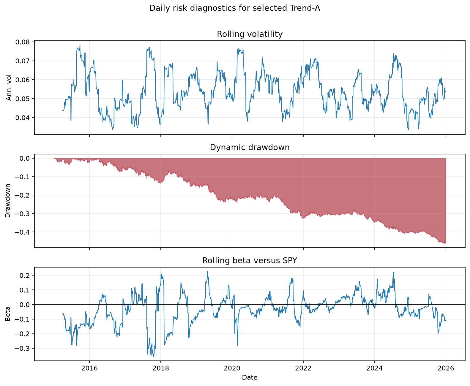
The figures that follow are from the Part 1 backtest daily series, not from IBKR Paper fills. Daily outputs feed Pyfolio [16], rolling VaR, rolling volatility, dynamic drawdown, and rolling SPY beta. This separates the custom backtest—which owns execution and costs—from the independent performance-reporting layer. Figure 13 summarises the daily risk path for the selected Trend-A strategy: rolling volatility remains elevated, dynamic drawdown deepens over multi-year stretches, and rolling SPY beta is unstable and often near zero or negative—consistent with a high-turnover rule that is not a simple long-equity clone. Figure 14 is the corresponding Pyfolio returns tear sheet exported from the same daily series.

9. Limitations
Minute-derived OHLCV bars do not contain the exchange tick sequence, quotes, queue priority, or order-book depth, so the event-bar study uses one-minute rows only as a sampling proxy. The fixed-basis-point cost model also omits time-varying spreads and market impact. Because QQQ is the only primary instrument, the results do not establish cross-asset robustness.
Hurst and variance-ratio estimates are noisy and respond slowly to regime changes; the inclusive OR gate used here therefore remains a soft screen, as quantified in Section 4.3. Cross-timeframe Sharpes in Section 5.4 are full-sample diagnostics under the 30-minute selected rule and must not be read as independent out-of-sample successes. Parameter trials remain a source of selection risk despite the chronological split and Deflated Sharpe adjustment [1,8–11,13]. Data provenance is another constraint: the third-party seller supplied neither independently verifiable exchange-level lineage nor a documented adjustment method, although the local files pass the integrity checks reported in Section 3.
MockBroker and historical replay test software behaviour, not broker execution. IBKR Paper adds an external check of socket behaviour, acknowledgements, and reconciliation, but its fills are simulated from the top of book and some order types differ from production [19].
10. Relative-Value Mean Reversion
After the primary single-asset Bollinger result failed both gross and net tests, the traded object was changed to a relative-value spread rather than adding further single-name gates. The hedge ratio $\hat\beta$ is estimated by train-only OLS on log prices,
$$ \log P^{\mathrm{QQQ}}_t = a + \hat\beta\log P^{\mathrm{SPY}}_t + e_t, $$
and held fixed thereafter. The traded object is the log spread $S_t=\log P^{\mathrm{QQQ}}_t-\hat\beta\log P^{\mathrm{SPY}}t$. Entry thresholds are either Bollinger bands on $S_t$ or rolling Ornstein–Uhlenbeck equilibrium bands $\hat\mu\pm z\hat\sigma{eq}$. Positions are the corresponding long/short hedge portfolio, not a QQQ-only filter. Selection remains train-only Sharpe; validation and test never choose parameters. Success required (i) positive test gross Sharpe and (ii) a test net mean not significantly negative after costs. The spread/OU framing follows standard practical treatments of mean-reverting pairs [20].
The selected 30-minute rule uses $\hat\beta\approx 1.53$, a 40-bar EWMA Bollinger envelope with $k=2$, and Hurst/VR entry gating (12 train trials). It fails the stated success criteria: test gross Sharpe is about −1.40, test net Sharpe is −2.04, and the two-sided mean-return p-value is 0.0004. Full-sample gross return is also negative (−19%), so costs are not the sole explanation. Holding the same $\hat\beta$ and parameters fixed, the rule remains weak on hourly data (test Sharpe ≈ −0.68) and near flat but still non-positive on daily data (test Sharpe ≈ −0.08). Relative-value mean reversion therefore does not reverse the primary negative conclusion under this design.
11. Conclusion
The tested transparent 30-minute strategies do not generate statistically robust net returns in QQQ over the 2023–2025 test period. EMA–MACD–ADX and the VWMA ratio fail their positive-alpha hypotheses; Hurst/VR gating improves Bollinger mean reversion relative to an ungated version, but the resulting strategy remains unprofitable. Transaction costs are a major cause of failure for the trend rules, while the mean-reversion rule also lacks gross profitability.
The full enhanced Bollinger rule reduces turnover, loss, and drawdown relative to the original MR-BB, but matched ablations attribute most of that improvement to the slower 40-bar EWMA centre rather than to BandWidth, Hurst/VR, or the 3.5-sigma extreme veto. In particular, removing the BandWidth gate improves test Sharpe from −0.803 to −0.253, while the extreme veto has almost no economic effect. Those enhanced ablations must not be read as reversing H3 on the original MR-BB specification, where the Hurst/VR OR gate still improves the test Sharpe relative to an ungated rule.
The QQQ–SPY spread experiment likewise fails its gross/net success criteria on 30-minute data and remains non-positive when the same rule is applied without re-optimisation to 1h and 1d bars. Further work should therefore emphasise better cost measurement and a real Paper session rather than additional single-name Bollinger gates.
The engineering results are more constructive. A relatively simple strategy can be embedded in an auditable execution architecture with deterministic order identity, explicit state transitions, independent execution/position reconciliation, fault injection, risk limits, and fail-closed recovery. This operational layer does not rescue a weak strategy, but it prevents broker and process failures from silently increasing risk.
Pros of the methods. Transparent rules and closed-form indicators make every signal auditable. Train-only selection, embargo bars, IC/DSR diagnostics, cost stress, and matched ablations separate statistical artefacts from economic claims. The same codebase carries the rules into a fail-closed broker path with reconciliation and sequencing.
Cons of the methods. Rolling Hurst/VR and short-bar IC estimates are high variance; the inclusive OR gate is a weak screen. Fixed basis-point costs and close-to-close PnL are coarse relative to true execution. Paper evidence stresses order lifecycle rather than a fill-rich live benchmark, and single-name QQQ results do not generalise by themselves.
11.1 Future Research
Future research should first test whether the negative results are specific to a single-asset intraday design. A point-in-time, survivorship-bias-controlled S&P 500 or Nasdaq-100 universe would permit a comparison of time-series, cross-sectional, and market-beta-residual momentum on hourly and daily bars [3,21]. The VIX futures term structure could be evaluated as a candidate conditioning variable rather than imposed as a deterministic switch between trend and mean-reversion strategies [22]. Any incremental value should be measured through declared ablations, an untouched test period, and trial counts incorporated into the Deflated Sharpe analysis [10,11].
The measurement layer should also move beyond one-minute OHLCV proxies and fixed basis-point costs. Volume and dollar bars can be reconstructed from independently verifiable trades and quotes, while depth-of-book data would permit order-flow imbalance, spread, depth, and queue-sensitive diagnostics [13,23]. Option-derived gamma exposure should be studied only if archived option chains, open interest, and calculation assumptions are reproducible. Execution costs could then use time-varying spreads and an empirically estimated participation/impact model [1,24]. Timestamped Paper sessions and tightly controlled small live orders could measure acknowledgement latency, fill probability, partial fills, and adverse selection. The objective would be to quantify—not claim to eliminate—the gap between simulated and realised execution while preserving the same train/validation/test discipline used in the present study.
References
[1] Harris, L. (2003) Trading and Exchanges: Market Microstructure for Practitioners. Oxford: Oxford University Press.
[2] Invesco (2026) Invesco QQQ ETF. Available at: https://www.invesco.com/qqq-etf/en/home.html (Accessed: 4 August 2026).
[3] Moskowitz, T.J., Ooi, Y.H. and Pedersen, L.H. (2012) ‘Time Series Momentum’, Journal of Financial Economics, 104(2), pp. 228–250. doi:10.1016/j.jfineco.2011.11.003.
[4] Carver, R. (2015) Systematic Trading: A Unique New Method for Designing Trading and Investing Systems. Petersfield: Harriman House.
[5] Appel, G. (2005) Technical Analysis: Power Tools for Active Investors. Upper Saddle River, NJ: Financial Times Prentice Hall.
[6] Wilder, J.W. (1978) New Concepts in Technical Trading Systems. Greensboro, NC: Trend Research.
[7] Bollinger, J. (2001) Bollinger on Bollinger Bands. New York: McGraw-Hill.
[8] Hurst, H.E. (1951) ‘Long-Term Storage Capacity of Reservoirs’, Transactions of the American Society of Civil Engineers, 116, pp. 770–799. doi:10.1061/TACEAT.0006518.
[9] Lo, A.W. and MacKinlay, A.C. (1988) ‘Stock Market Prices Do Not Follow Random Walks: Evidence from a Simple Specification Test’, The Review of Financial Studies, 1(1), pp. 41–66. doi:10.1093/rfs/1.1.41.
[10] Bailey, D.H. and López de Prado, M. (2014) ‘The Deflated Sharpe Ratio: Correcting for Selection Bias, Backtest Overfitting, and Non-Normality’, The Journal of Portfolio Management, 40(5), pp. 94–107. doi:10.3905/jpm.2014.40.5.094.
[11] Bailey, D.H., Borwein, J.M., López de Prado, M. and Zhu, Q.J. (2017) ‘The Probability of Backtest Overfitting’, The Journal of Computational Finance, 20(4), pp. 39–69. doi:10.21314/JCF.2016.322.
[12] CQF Institute (2026) Trend Following and Mean Reversion Trading: Final Project Brief. Unpublished course material.
[13] López de Prado, M. (2018) Advances in Financial Machine Learning. Hoboken, NJ: John Wiley & Sons.
[14] Jolliffe, I.T. (2002) Principal Component Analysis. 2nd edn. New York: Springer. doi:10.1007/b98835.
[15] Sharpe, W.F. (1966) ‘Mutual Fund Performance’, The Journal of Business, 39(S1), pp. 119–138. doi:10.1086/294846.
[16] Jansen, S. and contributors (2026) pyfolio-reloaded: Portfolio and Risk Analytics in Python. Available at: https://github.com/stefan-jansen/pyfolio-reloaded (Accessed: 31 July 2026).
[17] Interactive Brokers (2026) TWS API Documentation. Available at: https://interactivebrokers.github.io/tws-api/ (Accessed: 31 July 2026).
[18] ib-api-reloaded contributors (2026) ib_async: Python Sync/Async Framework for the Interactive Brokers API. Available at: https://github.com/ib-api-reloaded/ib_async/ (Accessed: 4 August 2026).
[19] Interactive Brokers (2026) Paper Trading vs Live Trading—What’s the Difference? Available at: https://www.interactivebrokers.com/campus/trading-lessons/paper-trading-vs-live-trading-whats-the-difference/ (Accessed: 4 August 2026).
[20] Chan, E.P. (2013) Algorithmic Trading: Winning Strategies and Their Rationale. Hoboken, NJ: John Wiley & Sons. doi:10.1002/9781118676998.
[21] Jegadeesh, N. and Titman, S. (1993) ‘Returns to Buying Winners and Selling Losers: Implications for Stock Market Efficiency’, The Journal of Finance, 48(1), pp. 65–91. doi:10.1111/j.1540-6261.1993.tb04702.x.
[22] Simon, D.P. and Campasano, J. (2014) ‘The VIX Futures Basis: Evidence and Trading Strategies’, The Journal of Derivatives, 21(3), pp. 54–69. doi:10.3905/jod.2014.21.3.054.
[23] Cont, R., Kukanov, A. and Stoikov, S. (2014) ‘The Price Impact of Order Book Events’, Journal of Financial Econometrics, 12(1), pp. 47–88. doi:10.1093/jjfinec/nbt003.
[24] Almgren, R., Thum, C., Hauptmann, E. and Li, H. (2005) ‘Direct Estimation of Equity Market Impact’, Risk, 18(7), pp. 58–62.