使用蒙特卡洛模拟对欧式与二元期权定价
1. 引言
本文在风险中性框架下,使用蒙特卡洛模拟研究欧式看涨期权与二元看涨期权的定价问题。根据资产定价基本定理,期权价值 $V(S,t)$ 等于风险中性测度 $\mathbb{Q}$ 下贴现支付的期望:
$$V(S, t) = e^{-r(T-t)} \mathbb{E}^\mathbb{Q} [\text{Payoff}(S_T)]$$
假设标的资产价格服从几何布朗运动(GBM),其随机微分方程(SDE)为: $$dS_t = r S_t dt + \sigma S_t dW_t$$ 其中,$r$ 为无风险利率,$\sigma$ 为波动率,$dW_t$ 为维纳过程增量。
为模拟资产路径,本文采用三种数值方法:
- Euler-Maruyama 方法:一阶离散近似。 $$S_{t+\Delta t} = S_t + r S_t \Delta t + \sigma S_t \sqrt{\Delta t} Z$$
- Milstein 方法:包含 Itô 展开修正的高阶近似。 $$S_{t+\Delta t} = S_t + r S_t \Delta t + \sigma S_t \sqrt{\Delta t} Z + \frac{1}{2}\sigma^2 S_t \Delta t (Z^2 - 1)$$
- GBM 闭式解:该 SDE 的精确终值解。 $$S_T = S_0 \exp\left((r - \frac{1}{2}\sigma^2)T + \sigma \sqrt{T} Z\right)$$
此外,我们考察了 对偶变量法(Antithetic Variates) 与 控制变量法(Control Variates) 两种方差缩减技术。
| |
2. 基础模型可视化:资产路径
| |
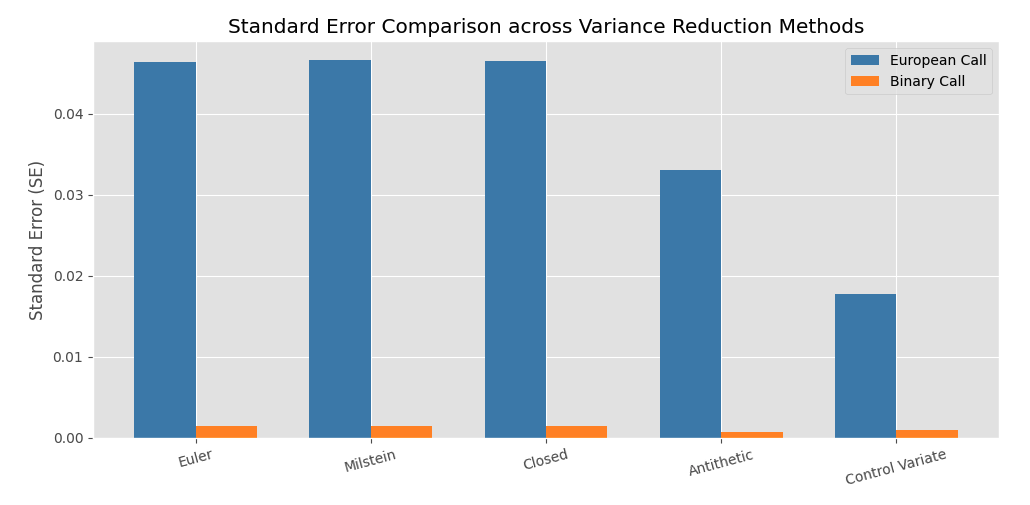
3. 结果:价格与标准误对比
| |
观察:方差缩减(VR)带来的效率提升
这一部分可以从四点来理解:
第一,关于离散化误差与采样效率:从 Euler 切换到 Milstein 主要改善的是离散化偏差,但对 标准误(SE) 的影响很小。结果显示 Euler、Milstein 与闭式解三者的 SE 基本接近。这说明 SE 主要由样本量($N$)与支付函数方差决定,而不是离散化格式本身。
第二,对偶变量法的表现:对偶变量法带来明显提升,欧式看涨的 VR 比率约 1.99x,二元看涨更高(约 4.64x)。通过构造负相关路径,它能抵消部分采样噪声,在相同计算预算下收窄置信区间。
第三,控制变量法(CV)的主导优势:在欧式看涨上,控制变量法效果最强,VR 比率约 6.88x。其核心是利用已知解析性质且与目标变量高度相关的控制变量(如标的终值)来显著降低剩余方差。
第四,支付函数敏感性:在本次实验中,对二元看涨而言,对偶变量法反而优于控制变量法(4.64 vs 2.45)。这表明 VR 技术效果对支付函数的不连续性与凸性高度敏感。
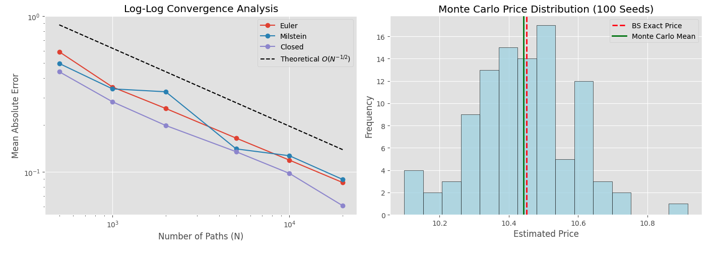
4. 收敛性与稳定性分析
| |
观察
第一张图说明了以下几点:
- 关于收敛速度与离散化偏差
- 理论收敛阶($O(N^{-1/2})$):log-log 图显示三种数值方法的误差下降轨迹都与理论参考线基本平行,经验上验证了蒙特卡洛估计方差符合中心极限定理。
- 离散化偏差:曲线之间的垂直间距揭示了时间离散误差。Euler 方法(一阶)绝对误差最大;Milstein 方法通过二阶 Itô 修正显著降低偏差;闭式解(精确 GBM)不存在时间离散偏差,剩余误差主要来自统计采样方差。
- 强收敛与弱收敛的权衡
- 路径精度(强收敛)角度:Milstein 通过考虑波动率拖曳项($1/2 \sigma^2 \dots$),使单条模拟路径更贴近“真实路径”,这对路径依赖产品(如美式、障碍期权)很关键。
- 分布统计(弱收敛)角度:对于整体统计量(如此处均值绝对误差),Milstein 相对 Euler 的优势可能有限,因为二者弱收敛阶同为 $O(\Delta t)$。在只看终值期望时,Milstein 的非线性修正有时会让结果在 Euler 附近波动。
- 实务选择:结果表明,若目标是简单欧式类期望定价,与其提升离散化复杂度,不如在标准 Euler 上结合方差缩减,往往更具计算效率。
第二张图可得:
- 100 个随机种子下的蒙特卡洛估计分布紧密围绕 Black-Scholes 精确值,样本均值(绿线)与解析基准(红线)高度一致,说明估计器无偏。
- 对称钟形直方图从可视化上验证了中心极限定理,也说明了蒙特卡洛的固有噪声,因此方差缩减对于提升效率非常关键。
5. 敏感性分析(参数变化)
| |
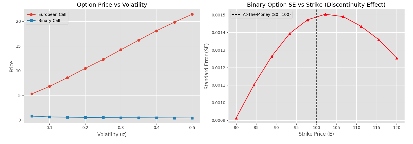
关于波动率敏感性图(Vega 分化)
- 敏感性分析显示出一个关键分化:随着隐含波动率上升,欧式看涨价格单调上升(正 Vega),而平值(ATM)二元看涨价格在本实验设置下下降(负向表现)。
- 对欧式期权而言,由于支付函数 $\max(S_T - E, 0)$ 的凸性,高不确定性带来的右尾扩张总体有利:上行收益不封顶、下行损失下限为 0。相反,ATM 二元期权支付上限固定为 1。波动率升高会把更多路径推向极端值,但上行额外空间被封顶,向下偏离却会完整损失支付,因此风险中性下实值概率被稀释,期望价值下降。
关于二元期权支付不连续性
- 二元期权的标准误(SE)在平值点($E = S_0 = 100$)附近显著抬升。
- 原因是其支付函数高度不连续(Heaviside 阶跃函数)。当模拟终值 $S_T$ 非常接近执行价 $E$ 时,极小随机扰动就会导致支付在 0 与 1 之间翻转,从而显著放大统计方差,使标准蒙特卡洛在 ATM 二元期权上效率明显低于连续支付的欧式期权。
6. 观察与遇到的问题
二元期权与欧式期权的差异:
- 观察: 二元期权的标准误(SE)行为与欧式期权明显不同。二元期权在平值(ATM,$E=100$)附近方差会出现尖峰。
- 原因: 这来自二元支付函数的强不连续性(从 0 到 1 的阶跃)。执行价附近路径的微小变动会引起支付结果的大幅跳变。
方差缩减效率:
- 控制变量法: 对欧式期权非常有效,方差缩减比(VRR)约为 7.0x(SE 约降低到原来的 $1/\sqrt{7}$)。其高效率来自 ATM 欧式支付 $\max(S_T - E, 0)$ 与连续控制变量 $S_T$ 之间较强的正相关($\rho \approx 0.92$)。
- 遇到的问题: 在二元期权上该效率显著下降。由于二元支付上限固定为 1,其与无界的 $S_T$ 线性相关性较弱,该控制变量对不连续数字支付的效果明显变差。
收敛与离散化:
- Log-Log 分析显示经验误差符合理论 $O(N^{-1/2})$ 收敛率。
- Euler 的时间离散偏差最大,Milstein 通过 Itô 修正提高了精度。
7. 结论
对于路径依赖型复杂衍生品,Euler 与 Milstein 仍是必要方法;但对路径无关的欧式与二元期权,GBM 闭式终值法由于完全消除了时间步进偏差,通常更优。
就方差缩减而言,基于标的终值 $S_T$ 的控制变量法在连续支付(欧式看涨)上效果非常强;但在不连续支付(二元看涨)上,线性关系减弱导致效率明显下降。
总结:数值方法不能“一套通吃”,应根据支付函数的数学结构(连续/不连续)进行针对性选择。
8. 参考文献
- Hull, J. C. (2018). Options, Futures, and Other Derivatives. Pearson.
- Glasserman, P. (2003). Monte Carlo Methods in Financial Engineering. Springer.
- Higham, D. J. (2001). “An Algorithmic Introduction to Numerical Simulation of Stochastic Differential Equations”. SIAM Review.